SharkFest 2014 - Packet Analysis and Visualization with SteelScript
This presentation was delivered at SharkFest on June 17, 2014 by
Christopher J. White. The source file
SharkFest2014.ipynb
is an IPython Notebook.
Overview
- Visualizing with SteelScript Application Framework
- Tools in my toolbox
- Python Pandas
- PCAP Analysis with SteelScript
SteelScript Application Framework
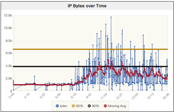
PCAP File: /ws/sharkfest2014/oneday.pcap
ip.lenfield over time- 95th and 80th percential
- Exponential Weighted Moving Average (EWMA)
Tools: IPython
- Powerful interactive shells (terminal and Qt-based).
- A browser-based notebook with support for code, text, mathematical expressions, inline plots and other rich media.
- Support for interactive data visualization and use of GUI toolkits.
- Flexible, embeddable interpreters to load into your own projects.
- Easy to use, high performance tools for parallel computing.
Installation
> pip install ipythonTools: pandas - Python Data Analysis Library
pandas is an open source, BSD-licensed library providing high-performance, easy-to-use data structures and data analysis tools for the Python programming language
- Series - array of data with an optional index
- DataFrame - 2D array of data hierarchical row and column indexing
Installation
Linux / Mac with dev tools?
> pip install pandasOtherwise see pandas.pydata.org
Tools: matlibplot - Python Plotting
matlibplot hooks in with IPython notebook to provide in browser graphs.
import numpy as np
import matplotlib.pyplot as plt

x = np.linspace(0, 2)
y = np.sin(4 * np.pi * x) * np.exp(-5 * x)

plt.fill(x, y, 'r')
plt.grid(True)
plt.show()

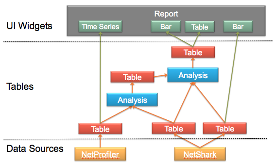
Tools: SteelScript Application Framework
- Web front end for simple user interface
- Design custom reports
- mix and match widgets and data
- define custom criteria
- Custom analysis via Python hooks and Python Pandas
- compute statistics, pivot tables, merge, sort, resample timeseries
- Plugin architecture makes it easy to share modules
pandas
Primary object types:
- Series - 1 dimensional array of element
- DataFrames - 2 dimensional array of elements
Data is stored is compact binary form for efficiency of operation.
Supports both row and column indexing by name.
pandas: Series
A Series is similar to a standard Python list, however much more efficient in memory and computation.
import pandas, numpy
s = pandas.Series([10, 23, 19, 15, 56, 15, 41])
print type(s)
s
s.sum(), s.min(), s.max(), s.mean()
Consider processing 1,000,000 random entries in a standard list:
%%time
s = list(numpy.random.randn(1000000))
%%time
print min(s), max(s), sum(s)
Now, consider processing 1,000,000 random entries in a pandas Series:
%%time
s = pandas.Series(numpy.random.randn(1000000))
len(s)
%%time
print s.min(), s.max(), s.sum()
del s
pandas: DataFrame
A DataFrame is typically loaded from a file, but my be created from a list of lists:
import pandas
df = pandas.DataFrame(
    [['Boston', '10.1.1.1', 10, 2356, 0.100],
     ['Boston', '10.1.1.2', 23, 16600, 0.112],
     ['Boston', '10.1.1.15', 19, 22600, 0.085],
     ['SanFran', '10.38.5.1', 15, 10550, 0.030],
     ['SanFran', '10.38.8.2', 56, 35000, 0.020],
     ['London', '192.168.4.6', 15, 3400, 0.130],
     ['London', '192.168.5.72', 41, 55000, 0.120]],
     columns = ['location', 'ip', 'pkts', 'bytes', 'rtt'])
Each column's data type is automatically detected based on contents.
df.dtypes
IPython has special support for displaying DataFrames
df
pandas: DataFrame operations
The DataFrame supports a number of operations directly
df.mean()
Notice that location and ip are string columns, thus there is no operation 'mean' for such columns.
df.sum()
In the case of sum(), it is possible to add strings, so location and ip are included in the results. (Be careful, on large data sets this can backfire!)
pandas: Selecting a Column
Each column of data in a DataFrame can be extracted by the standard indexing operator:
df[_colname_]The result is a Series.
df['location']
df['pkts']
pandas: Selecting Rows
Selecting a subset of rows based by index works just like array slicing:
df[_start_:_end_]Note that the : is always required, but <start> and <end> are optional. This will return all rows with an index greater than or equal to <start>, up to but not including <end>
df[:2]
df[2:4]
pandas: Filtering Rows
DataFrame rows can be filtered using boolean expressions
df[_boolean_expression_]df[df['location'] == 'Boston']
df[df['pkts'] < 20]
Expressions can be combined to provide more complex filtering:
df[(df['location'] == 'Boston') & (df['pkts'] < 20)]
The boolean expression is actually a Series of True/False values of the same length as the number of rows, thus can actually be assigned as a series:
bos = df['location'] == 'Boston'
print type(bos)
bos
pkts_lt_20 = (df['pkts'] < 20)
df[bos & pkts_lt_20]
Use single "&" and "|" and parenthesis for constructing arbitrary boolean expressions. Use "~" for negation.
The result of a filtering operation is a new DataFrame object
df2 = df[bos & pkts_lt_20]
print 'Length:', len(df2)
df2
pandas: Selecting Multiple Columns
A new DataFrame can be constructed from a subset of another DataFrame using the ix[] operator.
DataFrame.ix[_row_expr_,_column_lise_]locrtt = df.ix[:,['location', 'rtt']]
locrtt
The first argument to the ix[] indexer is actually expected to be a boolean Series. This makes it possible to select rows and columns in a single operation. The use of ":" above is short-hand for all rows.
boslocrtt = df.ix[bos,['location', 'rtt']]
boslocrtt
pandas: Adding Columns
New columns (Series) be added to a DataFrame in one of three ways:
- A constant value for all rows
- Supplying a
listmatching the number of rows - Expression based on constants and Series objects of the same size
df['co'] = 'RVBD'
df['proto'] = ['tcp', 'tcp', 'udp', 'udp', 'tcp', 'tcp', 'udp']
df['Bpp'] = df['bytes'] / df['pkts']   # Bytes per packet
df['bpp'] = 8 * df['bytes'] / df['pkts']
df['slow'] = df['rtt'] >= 0.1
df.ix[:,['ip', 'proto', 'Bpp', 'bpp', 'slow', 'delay', 'co']]
pandas: Grouping and Aggregating
A common operation is to group data by a key column or set of of key columns. The groups rows that share the same value for all key columns producing one row per unique key pair:
df.groupby(_key_columns_]For example, to group by the location column:
gb = df.groupby('location')
print type(gb)
gb.indices
The result of a grouping operation is a GroupBy object. The above indices shows you the row numbers for the grouped data. The data of a GroupBy object cannot be inspected directly until aggregated.
The groupby() operation is usually followed by an aggregate() call to combine the values of all related rows in each column.
In one form, the aggregate() call takes a dictionary indicating the operation to perform on each column to comine values:
GroupBy.aggregate({<colname>: <operation>,
                   <colname>: <operation>,
                   ... })
Only columns listed in the dictionary will be returned in the resulting DataFrame.
gb.aggregate({'pkts': 'sum',
              'rtt': 'mean'})
By copying columns, it is possible to compute alternate operations on the same data, producing different aggregated results:
df2 = df.ix[:,['location', 'pkts', 'rtt']]
df2['peak_rtt'] = df['rtt']
df2['min_rtt'] = df['rtt']
df2
agg = (df2.groupby('location')
          .aggregate({'pkts': 'sum',
                      'rtt': 'mean',
                      'peak_rtt': 'max',
                      'min_rtt': 'min'}))
agg
pandas: Indexing
Notice that the output of the preview groupby/aggregate operation looked a bit different from previous data frames, the first column is in bold:
agg
The bold rows/columns indicate that the DataFrame is indexed.
Let's look at the DataFrame without the index -- by calling reset_index():
agg.reset_index()
Indexing a DataFrame makes the data in the indexed column to meta-data associated with the object. This index is carried on to Series objects:
agg['pkts']
The resulting series still acts like an array, but may be indexed by either a numeric row value or a location name:
print "Boston:", agg['pkts']['Boston']
print "Item 0:", agg['pkts'][0]
df = df.ix[:,['location', 'ip', 'pkts', 'bytes', 'rtt', 'slow']]
pandas: Modifying a Subset of Rows
Often it is useful to assign a subset of rows in a column. This is possible by assigning a value to the result of the ix[] indexer:
DataFrame.ix[_row_expr_, _column_list_>] = <new value>When used in this form, the DataFrame object indexed is modified in place.
Let's use this method to assign a value of 'slow', 'normal', or 'fast' to a new 'delay' column based on rtt:
df['delay'] = ''
df
Compute boolean Series for each range of rtt:
slow_rows = (df['rtt'] > 0.110)
normal_rows = ((df['rtt'] > 0.050) & (~slow_rows))
fast_rows = ((~slow_rows) & (~normal_rows))
df.ix[slow_rows,'delay'] = 'slow'
df.ix[normal_rows, 'delay'] = 'normal'
df.ix[fast_rows, 'delay'] = 'fast'
df
pandas: Unstacking Data
Unstacking data is about pivoting data based on row values. For example, let's say we want to compute the total bytes for each delay category by location:
             slow   normal   fast
  Boston       ?       ?       ?
  SanFran      ?       ?       ?
  London       ?       ?       ?
Where the ? in each cell is the total bytes for that combination.
First we groupby both location and delay, aggregating the bytes column:
loc_delay_bytes = (df.groupby(['location', 'delay'])
                     .aggregate({'bytes': 'sum'}))
loc_delay_bytes
The resulting DataFrame has two index columns, location and delay.
Now the unstack() function is used to create a column for each unique value of delay:
loc_delay_bytes = loc_delay_bytes.unstack('delay')
Let's fill in zeros for the combinations that were not present:
loc_delay_bytes = loc_delay_bytes.fillna(0)
loc_delay_bytes
SteelScript for Python
SteelScript is a collection of Python packages that provide libraries for collecting, processing, and visualizing data from a variety of sources. Most packages focus on network performance.
Getting SteelScript and the Wireshark extension
Core SteelScript is available on PyPI:
> pip install steelscript
> pip install steelscript.wireshark
The bleeding edge is available on github:
- http://github.com/riverbed/steelscript/steelscript
- http://github.com/riverbed/steelscript/steelscript.wireshark
SteelScript: Reading Packet Capture Files
from steelscript.wireshark.core.pcap import PcapFile

pcap = PcapFile('/ws/traces/net-2009-11-18-17_35.pcap')
pcap.info()
print pcap.starttime
print pcap.endtime
print pcap.numpackets
Perform a query on the PCAP file
pdf = pcap.query(['frame.time_epoch', 'ip.src', 'ip.dst', 'ip.len', 'ip.proto'],
                starttime = pcap.starttime,
                duration='1min',
                as_dataframe=True)
pdf = pdf[~(pdf['ip.len'].isnull())]
print len(pdf), "packets loaded"
pdf[:10]
Examine some characteristics of the data:
pdf['ip.proto'].unique()
tcpdf = pdf[pdf['ip.proto'] == 6]
len(tcpdf)
Unique source IPs, or dest IPs:
pdf['ip.src'].unique()
pdf['ip.dst'].unique()
Examine the frame.time_epoch column:
s = pdf['frame.time_epoch']
s.describe()
SteelScript: Resampling
Pandas supports a number of functions specifically designed for time-series data. Resampling is particularly useful.
The current data set pdf contains one row per packet received over one minute. Let's compute the data rate in bits/sec at 1 second granularity.
Step 1 - Time Index
Resampling requires that DataFrame object have a datetime column as an index. The return value of the above pcap.query() autmatically converts the frame.time_epoch column into a datetime, now set it as the index:
print "frame.time_epoch:", pdf['frame.time_epoch'].dtype
pdf_indexed = pdf.set_index('frame.time_epoch')
Step 2 - Resample
Resample at 1second granularity, summing all ip.len values.
pdf_1sec = pdf_indexed.resample('1s', {'ip.len': 'sum'})
pdf_1sec.plot()

Step 3 - Compute bps
pdf_1sec['bps'] = pdf_1sec['ip.len'] * 8
pdf_1sec.plot(y='bps')

Defining Helper Functions
from steelscript.common.timeutils import parse_timedelta, timedelta_total_seconds

def query(pcap, starttime, duration):
    """Run a query to collect frame time and ip.len, filter for IP."""
    _df = pcap.query(['frame.time_epoch', 'ip.len'], \
                     starttime=pcap.starttime, duration=duration, \
                     as_dataframe=True)
    _df = _df[~(_df['ip.len'].isnull())]
    return _df
def plot_bps(_df, start, duration, resolution):
    """Plot bps for a dataframe over the given range and resolution."""
    # Filter the df to the requested time range
    end = start + parse_timedelta(duration)
    _df = _df[((_df['frame.time_epoch'] >= start) &
               (_df['frame.time_epoch'] < end))]

    # set the index
    _df = _df.set_index('frame.time_epoch')

    # convert a string resolution like '10s' into numeric seconds
    resolution = (timedelta_total_seconds(parse_timedelta(resolution)))

    # Resample
    _df = _df.resample('%ds' % resolution, {'ip.len': 'sum'})

    # Compute BPS
    _df['bps'] = _df['ip.len'] * 8 / float(resolution)

    # Plot the result
    _df.plot(y='bps')
%time pdf = query(pcap, starttime=pcap.starttime, duration='6h')
print len(pdf), "packets"
%time plot_bps(pdf, pcap.starttime, '6h', '15m')

%time plot_bps(pdf, pcap.starttime, '6h', '1m')

%time plot_bps(pdf, pcap.starttime, '1h', '1m')

%time plot_bps(pdf, pcap.starttime, '1h', '1s')

import datetime
from dateutil.parser import parse
import steelscript.wireshark.core.pcap
reload(steelscript.wireshark.core.pcap)
from steelscript.wireshark.core.pcap import *
SteelScript: Computing Client/Server Metrics
Now let's take a more complex example of rearranging the data.
- Incoming data is unidirectional data based on
src/dst - Determine
cli/srvbased on lower port number - Compute server-to-client (s2c) and client-to-server (c2s) bytes
- Rollup aggregate metrics
- Graph top 3 conversations
First, let's find the right field for port number. The TSharkFields class supports a find() method to look for fields by protocol, name, or description.
from steelscript.wireshark.core.pcap import TSharkFields, PcapFile

pcap = PcapFile('/ws/traces/net-2009-11-18-17_35.pcap')

tf = TSharkFields.instance()
tf.find(protocol='tcp', name_re='port')
Query the PCAP file for the necessary raw data, compute cli/srv/c2s/s2c:
%%time
pdf = pcap.query(['frame.time_epoch', 'ip.src', 'ip.dst', 'ip.len',
                  'tcp.srcport', 'tcp.dstport'],
                 starttime=pcap.starttime, duration='1m',
                 as_dataframe=True)
%%time
# Limit to TCP Traffic
istcp = ~(pdf['tcp.srcport'].isnull())
pdf = pdf[istcp]

# Assume lower port is the client
srccli = pdf['tcp.srcport'] > pdf['tcp.dstport']
%%time
# Initialize columns assuming server->client
pdf['ip.cli'] = pdf['ip.dst']
pdf['ip.srv'] = pdf['ip.src']
pdf['tcp.srvport'] = pdf['tcp.srcport']
pdf['c2s'] = 0
pdf['s2c'] = pdf['ip.len']
%%time
# Then override for client->server
pdf.ix[srccli, 'ip.cli']      = pdf.ix[srccli, 'ip.src']
pdf.ix[srccli, 'ip.srv']      = pdf.ix[srccli, 'ip.dst']
pdf.ix[srccli, 'tcp.srvport'] = pdf['tcp.dstport']
pdf.ix[srccli, 'c2s']         = pdf.ix[srccli, 'ip.len']
pdf.ix[srccli, 's2c']         = 0
Strip away the src/dst columns in favor of the cli/srv columns
pdf = pdf.ix[:, ['frame.time_epoch', 'ip.cli', 'ip.srv', 'tcp.srvport',
                 'ip.len', 'c2s', 's2c']]
pdf[:5]
Now, we can compute metrics for each unique host-pair:
cs = (pdf.groupby(['ip.cli', 'ip.srv', 'tcp.srvport'])
         .aggregate({'c2s': 'sum',
                     's2c': 'sum',
                     'ip.len': 'sum'}))
cs.sort('ip.len', ascending=False)[:10]
Pick the top 10 conversations, this will be used later for filtering:
top = cs.sort('ip.len', ascending=False)[:3]
top
Now, filter the original choosing only rows in the top 3:
cst = pdf.set_index(['ip.cli', 'ip.srv', 'tcp.srvport'])
cst_top = (cst[cst.index.isin(top.index)]
            .ix[:,['frame.time_epoch', 'ip.len']])
cst_top[:10]
Rollup the results into 1 second intervals
cst_top_time = (cst_top.reset_index()
                       .set_index(['frame.time_epoch', 'ip.cli', 'ip.srv', 'tcp.srvport'])
                       .unstack(['ip.cli', 'ip.srv', 'tcp.srvport'])
                       .resample('1s','sum')
                       .fillna(0))
cst_top_time.plot()

Questons?
Presentation available online:
- https://support.riverbed.com/apis/steelscript/SharkFest2014.slides.html
SteelScript for Python:
- https://support.riverbed.com/apis/steelscript/index.html